Learning representations of life

Monday. December 06, 2021 - 28 mins

I’m frequently asked how I think machine learning tools will change our approach to molecular and cell biology. This post is in part my answer and in part a reflection on Horace Freeland Judson’s history of early molecular biology – The Eighth Day of Creation.

Machine learning approaches are now an important component of the life scientist’s toolkit. From just a cursory review of the evidence, it’s clear that ML tools have enabled us to solve once intractable problems like genetic variant effect prediction¹, protein folding², and unknown perturbation inference³. As this new class of models enters more and more branches of life science, a natural tension has arisen between the empirical mode of inquiry enabled by ML and the traditional, analytical and heuristic approach of molecular biology. This tension is visible in the back-and-forth discourse over the role of ML in biology, with ML practitioners sometimes overstating the capabilities that models provide, and experimental biologists emphasizing the failure modes of ML models while often overlooking their strengths.

Reflecting on the history of molecular biology, it strikes me that the recent rise of ML tools is more of a return to form than a dramatic divergence from biological traditions that some discourse implies.

Molecular biology emerged from the convergence of physics and classical genetics, birthing a discipline that modeled complex biological phenomena from first principles where possible, and experimentally tested reductionist hypotheses where analytical exploration failed. Over time, our questions began to veer into the realm of complex systems that are less amenable to analytical modeling, and molecular biology became more and more of an experimental science.

Machine learning tools are only now enabling us to regain the model-driven mode of inquiry we lost during that inflection of complexity. Framed in the proper historical context, the ongoing convergence of computational and life sciences is a reprise of biology’s foundational epistemic tools, rather than the fall-from-grace too often proclaimed within our discipline.

Physicists & toy computers

Do your own homework. To truly use first principles, don’t rely on experts or previous work. Approach new problems with the mindset of a novice – Richard Feynman

When Linus Pauling began working to resolve the three-dimensional structures of the peptides, he built physical models of the proposed atomic configurations. Most young biology students have seen photos of Pauling beside his models, but their significance is rarely conveyed properly.

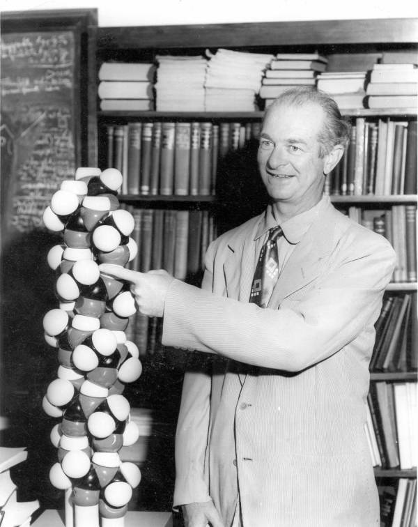
Pauling’s models were not merely a visualization tool to help him build intuitions for the molecular configurations of peptides. Rather, his models were precisely machined analog computers that allowed him to empirically evaluate hypotheses at high speed. The dimensions of the model components – bond lengths and angles – matched experimentally determined constants, so that by simply testing if a configuration fit in 3D space, he was able to determine if a particular structure was consistent with known chemistry.

These models “hard coded” known experimental data into a hypothesis testing framework, allowing Pauling to explore hypothesis space while implicitly obeying not only each individual experimental data point, but the emergent properties of their interactions. Famously, encoding the steric hindrance – i.e. “flatness” – of a double bond into his model enabled Pauling to discover the proper structure for the alpha-helix, while Max Perutz’s rival group incorrectly proposed alternative structures because their model hardware failed to account for this rule.

Following Pauling’s lead, Watson and Crick’s models of DNA structure adopted the same empirical hypothesis testing strategy. It’s usually omitted from textbooks that Watson and Crick proposed multiple alternative structures before settling on the double-helix. In their first such proposal, Rosalind Franklin highlighted something akin to a software error – the modelers had failed to encode a chemical rule about the balance of charges along the sugar backbone of DNA and proposed an impossible structure as a result.

Their discovery of the base pairing relationships emerged directly from empirical exploration with their physical model. Watson was originally convinced that bases should form homotypic pairs – A to A, T to T, etc. – across the two strands. Only when they built the model and found that the resulting “bulges” were incompatible with chemical rules did Watson and Crick realize that heterotypic pairs – our well known friends A to T, C to G – not only worked structurally, but confirmed Edwin Chargaff’s experimental ratios⁴.

These essential foundations of molecular biology were laid by empirical exploration of evidence based models, but they’re rarely found in our modern practice. Rather, we largely develop individual hypotheses based on intuitions and heuristics, then test those hypotheses directly in cumbersome experimental systems.

Where did the models go?

Emergent complexity in The Golden Era

The modern life sciences live in the shadow of The Golden Era of molecular biology. The Golden Era’s beginning is perhaps demarcated by Schroedinger’s publication of Max Delbrück’s questions and hypotheses on the nature of living systems in a lecture and pamphlet entitled What is Life?. The end is less clearly defined, but I’ll argue that the latter bookend might be set by the contemporaneous development of recombinant DNA technology by Boyer & Cohen in California ⁵ [1972] and DNA sequencing technology by Fredrick Sanger in the United Kingdom [1977].

In Francis Crick’s words⁶, The Golden Era was

concerned with the very large, long-chain biological molecules – the nucleic acids and proteins and their synthesis. Biologically, this means genes and their replication and expression, genes and the gene products.

Building on the classical biology of genetics, Golden Era biologists investigated biological questions through a reductionist framework. The inductive bias guiding most experiments was that high-level biological phenomena – heredity, differentiation, development, cell division – could be explained by the action of a relatively small number of molecules. From this inductive bias, the gold standard for “mechanism” in the life sciences was defined as a molecule that is necessary and sufficient to cause a biological phenomenon⁷.

Though molecular biology emerged from a model building past, the processes under investigation during the Golden Era were often too complex to model quantitatively with the tools of the day. While Pauling could build a useful, analog computer from first principles to interrogate structural hypotheses, most questions involving more than a single molecular species eluded this form of analytical attack.

The search to discover how genes are turned on and off in a cell offers a compact example of this complexity. Following the revelation of DNA structure and the DNA basis of heredity, Fraçois Jacob and Jacques Monod formulated a hypothesis that the levels of enzymes in individual cells were regulated by how much messenger RNA was produced from corresponding genes. Interrogating a hypothesis of this complexity was intractable through simple analog computers of the Pauling style. How would one even begin to ask which molecular species governed transcription, which DNA sequences conferred regulatory activity, and which products were produced in response to which stimuli using 1960’s methods?

Rather, Jacob and Monod turned to the classical toolkit of molecular biology. They proposed a hypothesis that specific DNA elements controlled the expression of genes in response to stimuli, then directly tested that hypothesis using a complex experimental system⁸. Modeling the underlying biology was so intractable that it was simply more efficient to test hypotheses in the real system than to explore in a simplified version.

The questions posed by molecular biology outpaced the measurement and computational technologies in complexity, beginning a long winter in the era of empirical models.

Learning the rules of life

John von Neumann […] asked, How does one state a theory of pattern vision? And he said, maybe the thing is that you can’t give a theory of pattern vision – but all you can do is to give a prescription for making a device that will see patterns!

In other words, where a science like physics works in terms of laws, or a science like molecular biology, to now, is stated in terms of mechanisms, maybe now what one has to begin to think of is algorithms. Recipes. Procedures. – Sydney Brenner⁹

Biology’s first models followed from the physical science tradition, building “up” from first principles to predict the behavior of more complex systems. As molecular biology entered The Golden Era, the systems of interest crossed a threshold of complexity, no longer amenable to this form of bottom up modeling. This intractability to analysis is the hallmark feature of complex systems.

There’s no general solution to modeling complex systems, but the computational sciences offer a tractable alternative to the analytical approach. Rather than beginning with a set of rules and attempting to predict emergent behavior, we can observe the emergent properties of a complex system and build models that capture the underlying rules. We might imagine this as a “top-down” approach to modeling, in contrast to the “bottom-up” approach of the physical tradition.

Whereas analytical modelers working on early structures had only a few experimental measurements to contend with – often just a few X-ray diffraction images – cellular and tissue systems within a complex organism might require orders of magnitude more data to properly describe. If we want to model how transcriptional regulators define cell types, we might need gene expression profiles of many distinct cell types in an organism. If we want to predict how a given genetic change might effect the morphology of a cell, we might similarly require images of cells with diverse genetic backgrounds. It’s simply not tractable for human-scale heuristics to reason through this sort large scale data and extract useful, quantitative rules of the system.

Machine learning tools address just this problem. By completing some task using these large datasets, we can distill relevant rules of the system into a compact collection of model parameters. These tasks might involve supervision, like predicting the genotype from our cell images above, or be purely unsupervised, like training an autoencoder to compress and decompress the gene expression profiles we mentioned. Given a trained model, machine learning tools then offer us a host of natural approaches for both inference and prediction.

Most of the groundbreaking work at the intersection of ML and biology has taken advantage of a category of methods known as representation learning. Representation learning methods fit parameters to transform raw measurements like images or expression profiles into a new, numeric represenatation that captures useful properties of the inputs. By exploring these representations and model behaviors, we can extract insights similar to those gained from testing atomic configurations with a carefully machined structure. This is a fairly abstract statement, but it becomes clear with a few concrete examples.

If we wish to train a model to predict cell types from gene expression profiles, a representation learning approach to the problem might first reduce the raw expression profiles into a compressed code – say, a 16-dimensional vector of numbers on the real line – that is nonetheless sufficient to distinguish one cell type from another¹⁰. One beautiful aspect of this approach is that the learned representations often reveal relationships between the observations that aren’t explicitly called for during training. For instance, our cell type classifier might naturally learn to group similar cell types near one another, revealing something akin to their lineage structure.

At first blush, learned representations are quite intellectually distant from Pauling’s first principles models of molecular structure. The implementation details and means of specifying the rules couldn’t be more distinct! Yet, the tasks these two classes of models enable are actually quite similar.

If we continue to explore the learned representation of our cell type classifier, we can use it to test hypotheses in much the same way Pauling, Crick, and countless others tested structural hypotheses with mechanical tools.

We might hypothesize that the gene expression program controlled by TF X helps define the identity of cell type A. To investigate this hypothesis, we might synthetically increase or decrease the expression of TF X and its target genes in real cell profiles, then ask how this perturbation changes our model’s prediction. If we find that the cell type prediction score for cell type A is correlated with TF X’s program more so than say, a background set of other TF programs, we might consider it a suggestive piece of evidence for our hypothesis.

This hypothesis exploration strategy is not so dissimilar from Pauling’s first principles models. Both have similar failure modes – if the rules encoded within the model are wrong, then the model might lend support to erroneous hypotheses.

In the analytical models of old, these failures most often arose from erroneous experimental data. ML models can fall prey to erroneous experimental evidence too, but also to spurrious relationships within the data. A learned representation might assume that an observed relationship between variables always holds true, implicitly connecting the variables in a causal graph, when in reality the variables just happened to correlate in the observations.

Regardless of how incorrect rules find their way into either type of model, the remedy is the same. Models are tools for hypothesis exploration and generation, and real-world experiments are still required for validation.

Old is new

Despite the implementation details, ML models are then not so distinct from the analog models of old. They enable researchers to rapidly test biological hypotheses to see if they obey the “rules” of the underlying system. The main distinction is how those rules are encoded.

In the classical, analytical models, rules emerged from individual experiments, were pruned heuristically by researchers, and then a larger working model was built-up from their aggregate. By contrast, machine learning models derive less explicit rules that are consistent with a large amount of experimental data. In both cases, these rules are not necessary correct, and researchers need to be wary of leading themselves astray based on faulty models. You need to be no more and no less cautious, no matter which modeling tool you choose to wield.

This distinction of how rules are derived is then rather small in the grand scheme. Incorporating machine learning models to answer a biological question is not a departure from the intellectual tradition that transformed biology from an observational practice to an explanatory and engineering disipline. Rather, applications of ML to biology are a return to the formal approaches that allowed molecular biology to blossom from the fields that came before it.

Footnotes

Jacob C. Kimmel

Co-founder & Head of Research @ NewLimit. Interested in aging, genomics, imaging, & machine learning.

Tweet Share