So You Want to Segment a Cell?
- 19 minsWhat is segmentation?
Segmentation is the act of discriminating foreground from background in an image or separating distinct regions.
In biological image analysis, this often distills down to discriminating objects or regions of interest like cells from uninteresting regions, like debris or background.
Segmentation is often one of the first steps in an image based cytometry pipeline. Before you can analyze a cell’s morphology, you need to find the cells in your image. For the rest of this post, I’ll demonstrate how to segment a brightfield cell image as an exercise for learning basic segmentation techniques.
What separates foreground from background?
Taking a step back, let’s think abstractly about how we determine whether a given region of an image is foreground or background – in this case, cell or plastic. It seems trivial because our brains perform recognition unconsciously, but if you focus you can describe the particular qualities that separate an apple from a fruit bowl, a child from a field of grass, or yes, a cell from plastic.
If we consider some of the qualities for our special case here, we might say that cells in brightfield images are darker than their background, with more diverse textures, and with specific shapes or structures inside. Imagine going pixel-by-pixel through an image and measuring how much of each of these qualities the pixel exhibits – darkness, texture relative to neighboring pixels, the presence of particular shapes. We could create a companion images of equal size for each of these qualities, where each pixel’s intensity represents not the number of photons captured by the detector, but our measurement of that particular quality.
These “companion images” are known as response maps or feature maps. They are often generated by convolving a filter that measures some desired property, and the resulting output is known as the response to the filter. Filtering to measure these properties of interest will be one of three primary tools we use for segmentation.
Let’s take a tour of those tools.
(1) Thresholding
Once we have a response map that tells us which sections of the image are more textured, which contain certain shapes, etc, how do we go about finding a cut-off for the foreground relative to the background?
Enter, thresholding.
Thresholding algorithms attempt to set a cut-off separating two modes of a distribution. What’s the simplest thresholding algorithm we can imagine? We could take the mean $\mu$ of the distribution of values $X$ in our response map and then simply classify values above the mean as foreground and values below as background. Such a simple algorithm doesn’t work very well in practice, but it gives you an idea for how thresholding works. Applying such an algorithm to the whole set of pixels in an image $X$ is known as global thresholding. As one might guess, there is also a concept of local thresholding, where thresholding algorithms are applied in the same manner, but considering subsets of pixels at a time in a series of “neighborhoods.”
The most common thresholding algorithm in image processing is Otsu’s algorithm applied globally, which minimizes the variance within the “classes” you’re separating, and maximizes the variance between them. Otsu’s method is implemented in most common image processing toolboxes, including in Matlab as graythresh and in Python’s scikit-image as skimage.filters.threshold_otsu. Several other thresholding algorithms exist and have common implementations. The scikit-image documentation has a nice overview.
(2) Filtering
In order to generate response maps for features other than simple brightness, we need to find a mathematical way of measuring our features of interest. As mentioned above, convolving an image with a specific filter kernel will generate a response map, so all we need to do is find a set of filter kernels that measure properties we’re interested in!
Understanding the mathematics behind two-dimensional convolution is really critical to understanding image processing, and I highly recommend reading up on the topic if you’re unfamiliar. Cornell’s CS Dept. has a nice tutorial and a live visual demonstration is available from Victor Powell.
Features of interest
Listed here are some common filters used for different features of interest in simple segmentation problems. There are many more, and each of these filters has multiple uses, but this list is a basic toolkit to help us get started.
| Feature | Kernel | |
|---|---|---|
| Blobs | Laplacian of Gaussian | |
| Brightness | N/A | N/A |
| Edges | Canny | |
| Edges | Sobel | |
| Edges | Gradient of Gaussian | |
| Texture | Combinations of Edge Filters |
(3) Morphological Operators
In addition to convolutions (i.e. filtering) and thresholding, morphological operators are the third leg of the stool that enables accurate segmentation.
At the most basic level, a morphological operation considers each pixel in an image and applies a non-linear transformation based on some rule. These rules usually consider some neighborhood of pixels around the center pixel, and apply a transform based on pixels in the neighborhood. The most common morphological operations are called dilation and erosion. We’ll walk through the details of each below.
Structuring Elements
How do we decide what the “neighborhood” around each pixel we’re transforming is? We use structuring elements.
Structuring elements are essentially shapes encoded as a binary matrix. So, if we want the neighborhood for morphological operation to be a disk with a radius $r$, we can generate a structuring element matrix that encodes a circle of True pixels. Using this disk structuring element, we can apply some transformation to each pixel in the image based on the neighboring pixels within the disk centered on the pixel to be transformed.
Let’s generate a structuring element using Python’s scikit-image and numpy toolsets.
# import some image processing functions and modules
from skimage.morphology import binary_erosion, binary_dilation, disk, square
import numpy as np
import matplotlib.pyplot as plt

# Look at some structuring elements
disk(10)
plt.imshow(disk(10), cmap='gray')
plt.show()
square(5)
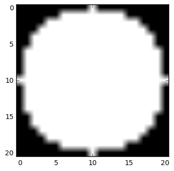
If we view the resulting plotted image, we get a nice disk!
Dilation
Dilation considers each pixel in an image and sets the value of this pixel to the maximum value of all pixels in a specified neighborhood. You can think of it sort of like a non-linear filter that applies a $\max$ operator rather than a convolution. So, it will set the value of each pixel to the highest pixel value within the neighborhood.
Whereas convolution is denoted with a $\star$, dilation is denoted with the operator $\oplus$. Mathematically, we denote the dilation of image matrix $I$ by structuring element $S$ as:
\[I \oplus S = \bigcup_{s \in S} I_s\]where $\bigcup$ is the union operator, denoting that our final dilated image is the union of structuring element sized “subimages” where I is transformed by the $\max$ operator with $S$. This can be intuitively understood as saying that the value of each pixel in the new transformed image is set based on the $\max$ value in the pixel’s neighborhood in the original image, i.e. we don’t transform part of the image “in place”, then consider those new transformed values for the next pixel over. Think of it like we make an empty copy of the image matrix, then fill it in pixel by pixel considering only the pixels of the original image.
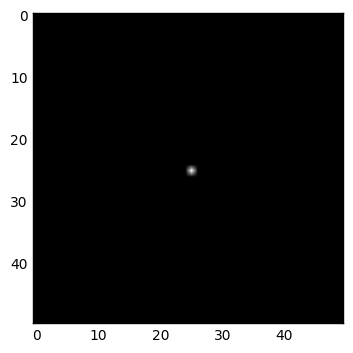
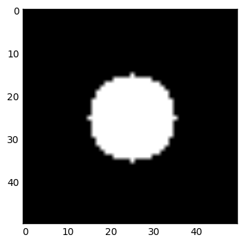
What does dilation look like in practice? Here, we perform dilation on a single pixel at the center of an image using a disk structuring element. You’ll see we create a disk! This makes intuitive sense, as when we scan across the image and perform the $\max$ operation
# Create a binary image with only 1 pixel 'True' at the center
I = np.zeros([50, 50])
I[I.shape[0]//2, I.shape[1]//2] = 1 # set center pixel to 1
# plot the image with matplotlib.pyplot.imshow()
plt.imshow(I, cmap='gray') # use the grayscale color map
plt.show()
# Now dilate the image with a disk structuring element
I_dil_disk = binary_dilation(I, selem=disk(10))
plt.imshow(I_dil_disk, cmap='gray')
plt.show()
Erosion
Now that we understand dilation, understanding erosion is easy.
Erosion considers each pixel in image and sets each pixel to the minimum value of all pixels in a neighborhood. Just like dilation, but instead of taking the $\max$ we’re taking the $\min$.
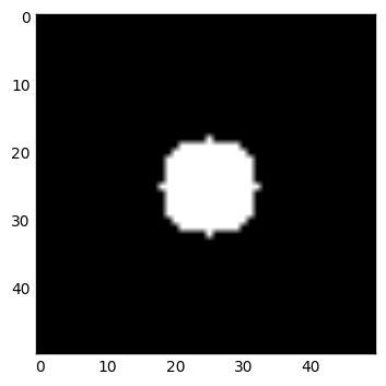
We can see how this works when we erode the images we just dilated.
# Let's erode some of those structuring elements we just dilated
I_erod_disk = binary_erosion(I_dil_disk, selem=disk(3))
plt.imshow(I_erod_disk, cmap='gray')
plt.show()
I_erod_square = binary_erosion(I_dil_square, selem=square(10))
plt.imshow(I_erod_square, cmap='gray')
plt.show()
Opening and Closing
It can be useful to perform a dilation followed by a corresponding erosion, and vice-versa. At first this seems a bit counterintuitive. Why perform two operations that leave us close to the starting point?
Eroding an image followed by a corresponding dilation (i.e. a dilation of similar magnitude and shape) is known as opening. This name comes from the fact that eroding tends to break thin “bridges” between binary objects. The subsequent dilation returns objects to roughly the same size as the starting point, but doesn’t restore these bridges, unlinking connected objects. You can think of it like “opening” a drawbridge linking two binary land masses. This is super useful in situations where a couple cells are just barely touching, letting you segment them individually.
Conversely, dilating an image followed by a corresponding erosion is known as closing. Two binary objects that are separated by a thin margin may form a connecting bridge when dilated, and the subsequent erosion may not break this bridge if it is thick enough. This “closes” the gaps between two objects.
As may be obvious, these dilation/erosion combinations are useful when you’re trying to separate touching cells, or connect parts of the same cell that might initially be separated in your segmentation.
In grayscale images, the same intuitions apply. Just think of opening as removing small high intensity connections between larger high intensity areas, and vice-versa for closing.
Lets create a bridge that we close, then open.
# Create a bridge to close and open with morphological operators
broken_bridge = np.zeros((50,50))
broken_bridge[24:26, 0:24] = 1
broken_bridge[24:26, 25:] = 1
plt.imshow(broken_bridge, cmap='gray')
plt.show()
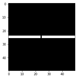
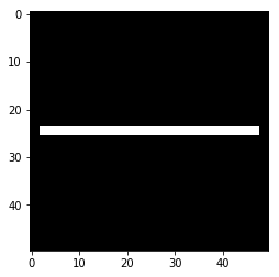
Let’s repair the middle using a morphological closing.
# Let's fix the bridge using morphological closing
# Here we use `binary_closing` and a disk structuring
# element `selem` to define the neighborhood
from skimage.morphology import binary_closing, binary_opening
fixed_bridge = binary_closing(broken_bridge, selem=square(5))
plt.imshow(fixed_bridge, cmap='gray')
plt.show()
# Notice, the erosion step at the end actually cuts off the bridge ends!
# Good thing no one will try and cross it :-D
Now let’s do some demolition instead and get a feel for how morphological opening can disconnect two objects with a small connection.
# Let's make another bridge, then break it
sacrificial_bridge = np.zeros((50,50))
sacrificial_bridge[22:30, 0:21] = 1
sacrificial_bridge[22:30, 30:] = 1
sacrificial_bridge[25:27, 21:30] = 1
plt.imshow(sacrificial_bridge, cmap='gray')
plt.show()
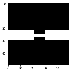
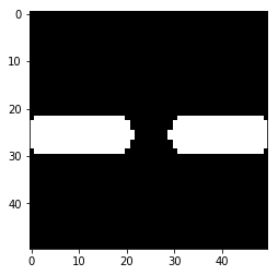
# Controlled demolition, using `binary_opening` with a small disk
# structuring element `selem` as the neighborhood
demolished_bridge = binary_opening(sacrificial_bridge, selem=disk(1))
plt.imshow(demolished_bridge, cmap='gray')
plt.show()
# Notice the corners of the bridge get "opened" too, since there are no
# + pixels off the edge of the image to recover those pieces when the dilation
# is performed
Segmenting a Cell Image
Now that we’ve taken a look through the tool box, here’s our challenge: create a binary “mask” that labels pixels representing a cell as $1$ and pixels labeling background as $0$ in this image of a muscle stem cell (MuSC) taken in DIC.

When we’re done, we’ll have a mask that looks like this.
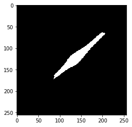
As you can see, it separates the cell from the background quite nicely.
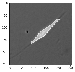
Start with Edges
When beginning any cell segmentation problem, it’s prudent to start by trying to identify the cell edges. In low contrast images this doesn’t always work so well, but it’s a great start if you can find a reliable algorithm to outline each cell.
In the example image we’re using, our DIC imaging provided a nice ‘halo’ around the cell edge, making it very distinct.
Sobel’s edge finding algorithm is an old-school, reliable place to start. As noted above, Sobel’s edge finding algorithm is a convolution of our image I with a 3x3 kernel that identifies areas with one bright side, and one dark side – an edge!
scikit-image has a handy sobel function, but let’s do this from scratch to remove some of the magic.
# Build Sobel filter for the x dimension
s_x = np.array([[1, 0, -1],
                [2, 0, -2],
                [1, 0, -1]])
# Build a Sobel filter for the y dimension
s_y = s_x.T # transposes the matrix
print(s_x)
print(s_y)
This will return our filters. Notice how s_x finds edges with bright pixels on one side, and dimmer pixels on the other, and the same for s_y in the vertical direction.
# s_x
[[ 1  0 -1]
 [ 2  0 -2]
 [ 1  0 -1]]

# s_y
[[ 1  2  1]
 [ 0  0  0]
 [-1 -2 -1]]
Now, we just convolve our image I with both kernels and add the responses together to estimate the gradient G. Note, we’re only checking the kernels in one direction. This means s_x responds with positive values for edges that are bright on the left, dark on the right, and negative values for edges that are dark on the left, bright on the right. All we need to do to account for this is square both responses and calculate the gradient G as the square root of their sum.
# Convolve with s_x and s_y
from scipy.ndimage.filters import convolve

res_x = convolve(I, s_x)
res_y = convolve(I, s_y)

# square the responses, to capture both sides of each edge
G = np.sqrt(res_x**2 + res_y**2)
plt.imshow(G, cmap='gray')
plt.show()
Look how well that worked!
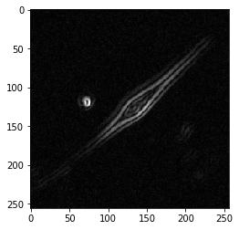
Let’s double check we did it properly using the scikit-image implementation.
# Let's check that our homemade version is the same
# as the result from the sobel() function
# made by the pros
from skimage.filters import sobel
I_edges = sobel(I)
plt.imshow(I_edges, cmap='gray')
plt.show()
You’ll see it looks the same!
Make a binary image
So, now we have an outline of the cell, but we need to get from our intensity image to a simple binary – 1 for edges, and 0 for everything else.
Otsu’s threshold as described above is perfect for this task. Let’s try it out.
# Threshold on edges
from skimage.filters import threshold_otsu

threshold_level = threshold_otsu(G)
bw = G > threshold_level # bw is a standard variable name for binary images

threshold_level

plt.imshow(bw, cmap='gray')
plt.show()
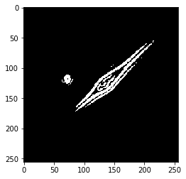
You’ll see there’s some grainy noise in the image. Let’s clear small objects to get rid of this.
# Let's clear any small object noise
from skimage.morphology import remove_small_objects
bw_cleared = remove_small_objects(bw, 300) # clear objects <300 px
plt.imshow(bw_cleared, cmap='gray')
plt.show()
Fill in the Gaps
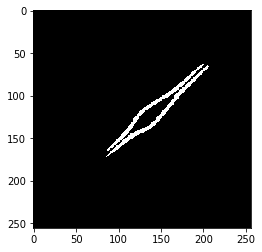
Now let’s use morphological closing to connect the gaps between edges.
# Let's close the edges of the outline with morphological closing
bw_close = binary_closing(bw_cleared, selem=disk(5))
plt.imshow(bw_close, cmap='gray')
plt.show()
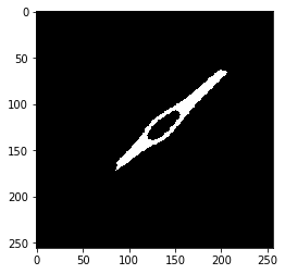
That looks pretty good! Now let’s fill in that one hole in the center. This uses one of the binary tools from scipy.ndimage.
# Now let's fill in the holes
from scipy.ndimage import binary_fill_holes
bw_fill = binary_fill_holes(bw_close)
plt.imshow(bw_fill, cmap='gray')
plt.show()

That looks pretty good! Let’s look at an overlay to make sure.
# Plot an overlay of our binary image
f = plt.figure()
plt.imshow(I, cmap='gray', interpolation=None)
plt.imshow(bw_fill, cmap='gray', alpha=0.5, interpolation=None)
plt.show()
# Not bad!

Conclusion
We’ve now walked through how to segment a cell using the bread and butter tools of traditional image analysis. Scenarios in the real world are often much more difficult than this toy example, but the approaches and concepts are largely the same. It’s amazing how much you can do with just these simple tools – convolution, thresholding, and morphological operators.
